
About the Scenario Tool
On this page, you will find an in-depth presentation of how climate change has affected Sweden on multiple levels up until 2018, as well as how these changes may develop throughout the 21st century. Our visualisation service is based on advanced scenarios from a range of climate models, both regional and global.
Climate models
To project future climates, climate models are used, offering three-dimensional representations of the atmosphere, land surface, oceans, lakes, and ice. These models are divided into a grid that spans the Earth's surface and extends upwards into the air, and in some cases, down into the ocean. When models include the entire atmosphere, and sometimes the oceans as well, they are referred to as global climate models. In each grid point, the evolution over time of various meteorological, climatological, and, in some cases, oceanographic parameters is calculated.
To achieve more detailed results, the horizontal resolution of the regional models has been increased from 50 km to 12.5 km. These regional models are based on information about future changes in the atmosphere and handle the interactions between physical processes in the atmosphere, on land, and in the ocean. The results from the climate models are processed further for each county in Sweden and cover the period from 1951 to 2100. Climate model calculations are part of the international research programmes CORDEX (cordex.org) and the Copernicus Climate Change Service (climate.copernicus.eu).
Climate models generate a vast amount of information and therefore require significant computing power. This means that the three-dimensional grid must be limited, which often leads to a relatively coarse grid in global climate models, resulting in less detail at the regional scale. To increase the level of detail for smaller geographic areas, such as Europe, regional climate models are used. These have a denser grid and can thus provide more detailed forecasts for specific regions without requiring excessive computing power.
The results outside the computational domain of a regional climate model are controlled by the output from a global climate model, ensuring that changes occurring outside the area are also taken into account. In climate models for Europe, a resolution of approximately 12.5 x 12.5 km is used in the horizontal grid.
High-resolution climate modelling is therefore very resource-intensive, but through a process known as downscaling, more detail and better results can be achieved. The higher resolution provides more data points, resulting in more detailed outcomes and better representation of climatological processes. This is particularly true for short and local events, as high-resolution models describe these better than low-resolution models. Precipitation, in general, and extreme precipitation, in particular, are examples of phenomena that are improved with higher resolution. Precipitation can vary significantly in both time and space, which is better represented by a high-resolution model (Rummukainen, 2010; Rummukainen, 2016).
In the ocean, high resolution is also necessary to describe flows in straits, such as the Öresund and the Great Belt, which are important for the climate and environment of the Baltic Sea.
Specific to Oceanography
In ocean climate models, both the atmosphere and the ocean are divided into three-dimensional grids that extend down into the ocean. These models calculate the evolution over time of both meteorological and oceanographic parameters. In coastal areas, the ocean requires a higher resolution than the atmosphere to capture detailed changes. For these areas, a resolution of approximately 3.7 x 3.7 km is often used for the ocean, while the atmospheric resolution may be around 25 x 25 km over the land surface.

Figure.A global model is required to simulate the climate. By modelling only a portion of the Earth in a regional model, higher detail can be achieved, but this requires data from a global model. Additional calculations and modelling may be needed, such as calculating indicators, ocean currents, or modelling connectivity, among other factors.
Emission scenarios
Climate model calculations are based on emission scenarios (or radiative scenarios). Emission scenarios are assumptions about future greenhouse gas emissions. They are based on projections of the future development of the global economy, population growth, globalisation, the transition to environmentally friendly technology, and more. All these factors influence the magnitude of greenhouse gas emissions, which in turn affect the greenhouse effect.
A measure of how the greenhouse effect will change in the future is radiative forcing, measured in watts per square metre (W/m²). The higher the greenhouse gas emissions, the greater the radiative forcing. Such scenarios are called RCP scenarios (Representative Concentration Pathways) (Moss et al., 2010; van Vuuren et al., 2011).
In this analysis, three scenarios are used:
- RCP2.6: Strong climate policies cause greenhouse gas emissions to peak in 2020, with radiative forcing reaching 2.6 W/m² by 2100. This scenario aligns most closely with the ambitions of the Paris Agreement and is used for meteorological and hydrological indicators. However, a complete analysis for oceanographic indicators is lacking for RCP2.6, so it is not included in the visualisation service for Swedish seas.
- RCP4.5: Strategies for reduced greenhouse gas emissions result in radiative forcing stabilising at 4.5 W/m² before 2100.
- RCP8.5: Increasing greenhouse gas emissions lead to radiative forcing reaching 8.5 W/m² by 2100 (as used in IPCC, AR5).
Climate scenarios
A climate scenario is created by combining an emission or radiative scenario, a global climate model, a regional climate model, and the chosen time period. See the table in the ensemble section for more information on the climate models used.
The regional models start at different times depending on the model, between 1951 and 1975. Climate calculations use a reference period of 1971–2000 (or 1976–2005, depending on the source) to describe how the climate changes over time. Future projections show deviations from the average of this reference period.
Since the results from the calculations are presented in a grid (or a three-dimensional grid), it can be challenging to directly compare model results with observations. Observations provide climate data for specific locations, while models provide average values for the entire grid cell. The description of observed climate in this service is based on gridded data (or reanalysis data in a three-dimensional grid, a combination of model and observational data), which facilitates comparison with the climate model data.
Reference data
Our service offers a comprehensive set of reference data for meteorology, hydrology, and oceanography, enabling detailed analysis and comparison of climate and water variables.
For meteorological data, we use SMHI's reference dataset for climate (SMHI GridClim), which covers the periods from 1961 to 2018. This dataset compiles daily observations of mean temperature, maximum and minimum daily temperatures, and daily precipitation from over 900 weather stations in Sweden and more than 2,000 precipitation stations, as well as observations from neighbouring countries. To fill gaps in areas without observation stations, we use a "first guess" based on UERRA regional reanalysis, which is a historical 3D simulation of the atmosphere. By downscaling the reanalysis from 11 km to 2.5 km horizontal resolution and combining it with station data, we optimise the interpolation of climate variables, creating a realistic representation on a grid over Scandinavia. This dataset is used to calculate climate indicators, analyse climate change, and bias-adjust climate models.
In hydrology, we use the reference dataset PTHBV (Johansson and Chen, 2003), which consists of daily observations of precipitation and temperature for Sweden on a grid with a resolution of 4x4 km². The dataset is calibrated to accurately represent streamflow and is also used for bias-adjustment of climate models for hydrological simulations.
For oceanographic data, we use a regional reanalysis performed by SMHI for the Copernicus Marine Service (CMEMS). The reanalysis is a historical calculation of the ocean in a three-dimensional grid, based on both surface and depth observations. Using the coupled physical-biogeochemical model NEMO-SCOBI, which has the same resolution as the regional climate models for the ocean, we obtain realistic values for climate variables. Reanalysis data for biogeochemical indicators are not yet available but will be included once methods are developed to address known issues, such as the high concentrations of dissolved inorganic nitrogen in the Gulf of Riga. These data can be accessed from Copernicus’ marine service (CMEMS).
Why are different reference periods used?
To describe the current climate, the most recent completed 30-year period, which is 1991–2020, is used. This period is representative of the current climate and provides an up-to-date picture of climate conditions. When describing older climate conditions or studying climate change, other reference periods may be chosen. The reference period 1961–1990 is commonly used for analysing climate changes, according to WMO guidelines. In some cases, other periods, such as the pre-industrial era, may be relevant depending on the research question.
In the early 2000s, the period 1961–1990 was not entirely representative of the then-current climate, and it was too early to use the subsequent period, 1991–2020. Therefore, the most recent 20–30 years were sometimes used as a reference period for comparing projected climate changes. When selecting reference periods, practical considerations such as data availability and the need to conserve computing power for climate model simulations are also important. Climate models may sometimes start after 1961, and the period 1971–2000 is often used as a compromise between computing power and historical reference.
In ocean analysis, a 30-year period, in this case 1976–2005, is used to describe the ocean’s current state. This period was chosen because it had the most up-to-date available forcing data (boundary conditions) at the time of analysis, and to ensure that natural variability does not unduly influence the results.
Nutrient scenarios
For biogeochemical indicators, various nutrient scenarios have been used in addition to climate scenarios. These are:
- Base: Assumes no additional measures are taken, compared to current efforts, to reduce emissions from sources such as agriculture and water treatment. However, climate change leads to a gradual increase in nutrient input. The amount of nutrients reaching the Baltic Sea is therefore only influenced by the climate's impact on runoff.
- Low: Represents a reduction in nutrient input, where by 2020, levels have been lowered to those agreed upon by the Baltic Sea countries through the HELCOM collaboration, known as the Baltic Sea Action Plan (HELCOM, 2007, 2013).
- High: Represents an increase in nutrient concentrations from water inflow and the atmosphere, reflecting changes such as population growth and agriculture. Nutrient loads to the sea are thus influenced by both lifestyle and the impact of climate change on land runoff.
Scenarios are not forecasts
The results presented from climate model calculations are called climate scenarios, not forecasts. Climate scenarios are based on assumptions about future greenhouse gas emissions and concentrations, representing the statistical behaviour of weather and the ocean over a longer time—i.e., the climate. In contrast, a weather or ocean forecast provides information about what will happen over the coming days.
Bias adjustment
The complex climate system, with many interdependent processes that are not always fully understood or represented in climate models, inevitably leads to systematic deviations from observed values. These deviations can vary for different variables and regions worldwide.
Often, these deviations pose no issue when calculating climate indicators focused on the differences between a historical and a future scenario. However, certain indicators rely on absolute thresholds, such as the number of frost days, tropical nights, or precipitation above a certain level. Impact modelling, such as hydrological calculations, can also be affected by bias—for instance, whether water is stored as snow or flows into rivers as rainfall depending on potential bias near the freezing point.
A systematic deviation from observations, known as bias, in the climate model can skew these indicators, leading to misleading interpretations. To address such issues, the scenario service uses the bias-adjustment method MIdAS (MultI-scale bias AdjuStment; Berg et al., 2021, 2022). MIdAS was developed at SMHI and has been carefully evaluated with positive results compared to international state-of-the-art practices, where bias adjustment is applied as a necessary step before impact modelling. For the historical period, an algorithm adjusts all model values to align with observations, adjusting everything from low values and averages to high values. The same algorithm is then applied to future scenarios, making them well-suited for impact modelling and indicator production.
Calculation of "End of the Century"
The term "end of the century" refers to 2071–2100 to ensure a consistent timeframe across different disciplines—meteorology, hydrology, and oceanography. Although oceanographic calculations do not always extend to 31 December 2100—they typically end on 31 December 2099 for most models and 2097 for one—this is practically a minor issue. The few missing years from some ensemble members are assumed to have a marginal effect on the ensemble mean for 2071–2100.
Different reference periods
The reference period may be different in the different RCP scenarios even though they describe the same climate. The reason is that the ensembles have different sizes. The calculated ensemble mean is different because different numbers of simulations are used. The deviations are small and without significance.
About ensembles
An ensemble is a collection of different calculations of the future climate. These calculations can, for instance, differ in terms of the choice of climate model or emissions and radiation scenario, or nutrient scenario. A calculation included in an ensemble is referred to as an ensemble member. In oceanography, nutrient scenarios are also included as a complement to the climate scenarios.
Why should one use model ensembles?
An ensemble provides a good overview of the variation between different climate and nutrient scenarios and highlights uncertainties associated with simulating future conditions. The ensemble thus offers a measure of the reliability of the results. If many scenarios produce similar outcomes, the relative confidence in the results increases compared to if they were pointing in different directions.
One type of ensemble contains members calculated with different global and/or regional climate models but using the same emissions or radiation scenario. Differences in results arise because the various climate models represent the physical processes in the simulated climate system in different ways.
This demonstrates the uncertainties associated with our understanding of how the climate system works. Sometimes, the choice of global model has the greatest impact on the simulated climate, for example, when the climate is primarily influenced by large-scale atmospheric movements, such as in winter temperatures.
In contrast, summer precipitation is primarily governed by local cloud formation, so the choice of regional model becomes more crucial for the simulated climate (Kjellström et al., 2018; Sørland et al., 2018). In other words, selecting which climate models to include in an ensemble is not straightforward.
A model may perform well over some regions of the world but less well over others. Another model might accurately describe temperature but be less accurate with precipitation. Thus, large ensembles are valuable as they better represent the reliability of the results. In practice, the choice of ensemble is largely determined by how many and which model simulations are practically feasible.
Another type of ensemble is created by using a single global climate model with different model runs based on different initial conditions, which introduces small but plausible variations in the model's starting values. Given that both climate models and the climate system are inherently chaotic, a small difference at one point can lead to a significant difference at a later time. This approach allows for the study of the natural variability of the climate system.
Natural variability is important in the short term perspective
In addition to human influence on the climate, the climate system has its own natural variability. These natural fluctuations from year to year, or from one decade to another, complicate the analysis of climate scenarios. This is particularly true when studying climate changes over shorter timescales. By the year 2100, climate changes compared to today are projected to be so significant that trends will be clear, even though values may vary greatly from year to year.
With current knowledge, the natural variability of the climate cannot be predicted exactly (e.g., for a specific date). However, natural variability can be studied by creating an ensemble of multiple climate scenarios based on a radiation scenario but with different initial conditions. By the end of the century, uncertainty primarily depends on the choice of global climate model, radiation scenario, and for biogeochemical indicators, the chosen nutrient scenario.
Ensembles describe the reliability of the results
In an ensemble analysis, the spread of results provides an indication of how reliable these results are. Depending on the type of ensemble created, it is also possible to study the significance of the choice of climate model versus initial conditions.
This service presents two measures of robustness and spread: the proportion of models showing an increase and the standard deviation.
The proportion of models showing an increase indicates the fraction of the model ensemble that predicts an increase in the chosen index. If many models agree that something is increasing (or decreasing), it is considered a robust result. If the models disagree, the result is less robust.
The standard deviation measures the spread between models. Even if all models show an increase, the magnitude of the increase may vary between models. A large difference between models results in a high standard deviation, while a small difference results in a low standard deviation. The standard deviation can also be compared with the size of the change. If the change is small compared to the standard deviation, the magnitude of the change is not considered robust.
The number of models and scenarios used in an ensemble partially depends on the time period over which the climate is to be studied. Generally, the closer in time (a few decades) and the more extreme the situation addressed, the greater the need for a large array of different combinations of models and model initial conditions. In contrast, if the question pertains to a longer time horizon (centuries), there is a greater need for more scenarios that represent various possible future developments.
Meteorology
For the meteorological sections of the climate scenario service, comparison material is presented in the form of maps based on a combination of observations and reanalyses for the period 1961-2018, compiled in SMHI's reference dataset. This dataset (SMHI GridClim, an optimised combination of station data and the UERRA reanalysis) includes, among other things, daily mean temperature, daily maximum and minimum temperatures, and daily precipitation on a 2.5 km grid covering Scandinavia.
Indicators
In addition to temperature and precipitation a number of so-called climate indicators are calculated. Indicators are calculated from ordinary meteorological parameters. It may be the number of cold or hot days, accumulated precipitation of a week or the length of the vegetation period. Since many indicators are based on thresholds (for example when temperature exceeds a certain limit) they are sensitive to systematic deviations in the climate models. For example, if a model is a bit too cold it can have a large impact on the number of hot days. The calculations of indicators are thus based on bias adjusted data (see section on bias adjustment).
Definitions of the indicators
Name | Definition | Unit |
|---|---|---|
Temperature | Daily average temperature | °C |
Maximum temperature | Daily maximum temperature | °C |
Minimum temperature | Daily minimum temperature | °C |
Precipitation | Average precipitation | mm/mon |
Diurnal temperature range | Maximum temperature minus minimum temperature | °C |
Cooling degree days | Degree days with average temperature > 20 °C | Degree days |
Heating degree days | Degree days with average temperature < 17 °C | Degree days |
Zero crossings | Number of days with maximum temperature > 0 °C and minimum temperature < 0 °C | Number of days |
Frost days | Number of days with minimum temperature < 0 ºC | Number of days |
Days with heavy precipitation | Number of days with precipitation > 10 mm/day | Number of days |
Days with extreme precipitation | Number of days with precipitation > 25 mm/day | Number of days |
Dry days | Number of days with precipitation < 1 mm | Number of days |
Longest dry period | Longest consecutive period with precipitation < 1 mm/day | Number of days |
Start of vegetation period | The first day of the first consecutive six-day period where all six days have daily average temperatures > 5 °C | Day number |
End of vegetation period | The first day of the first consecutive six-day period where all six days have daily average temperatures < 5 °C after 1 July | Day number |
Length of vegetation period | The number of days from the start of the vegetation period until and including the end of the vegetation period | Number of days |
Summer days | Number of days with maximum temperature > 25 °C | Number of days |
Longest period of summer days | Longest consecutive period with summer days (maximum temperature > 25 °C) | Number of days |
Tropical days | Number of days with minimum temperature > 20 °C | Number of days |
Cold days | Number of days with maximum temperature < -7 °C | Number of days |
The principle is to use as many model simulations as possible, since more data give a better statistical foundation. It is also desirable with ensembles that do not lean too much on specific models. In that case certain models get a disproportionate significance. It may also be desirable that the RCP ensembles is of comparable sizes. The supply of simulations of RCP8.5 is significantly larger than for the other RCPs. There are also model combinations that have only been run for one or two RCPs. Since we want as big ensembles as possible, we will have to accept that the ensembles are not containing exactly the same models. Global models used by only a small number of RCMs and for only one RCP are omitted so that they do not contribute to the skewness between the ensembles.
Models included in the ensemble. The numbers 26, 45, 85 are notations for the scenarios RCP2.6; RCP4.5 and RCP8.5, respectively. The notations r1, r3, r12 indicate that the same global model is run with different initial conditions.
Hydrology
The hydrological model describes how water flows through the soil, lakes, and rivers and how much water is returned to the atmosphere through evaporation or flows out to the seas. This is calculated for approximately 40,000 sub-catchments in Sweden, but is presented in an overview format for 262 named areas in the display service.
Indicators
Hydrological climate indicators are calculated from standard hydrological parameters, such as river discharge.
Name | Definition | Unit |
|---|---|---|
Low flow days | Number of days with river discharge < the mean low flow, which is defined as the mean of the day with the lowest river discharge of each year in 1971-2000. | days |
Low soil moisture days | Number of days with soil moisture < the mean low soil moisture, which is defined as the mean of the day with the lowest soil moisture of each year in 1971-2000. | days |
Effektive precipitation (mean) | The difference between precipitation and evapotranspiration from the ground and canopy over the day. Presented as the mean over the period, and the geographical area. | mm/month |
Air temperature (mean) | The mean air temperature at 2m above the surface for the selected period, and the geographical area. | °C |
Runoff (mean) | Runoff for the selected period, and the geographical area. | mm/month |
Soil moisture (mean) | Mean soil mositure for the selected period, and the geographical area. | Unitless |
Precipitation (mean) | Mean precipitation for the selected period, and the geographical area. | mm/day |
River discharge (mean) | Mean river discharge for the selected period, and the geographical area. | m3/s |
Flood recurrence (2,5,10, or 50-yr) | The return level of river discharge for the selected return period, selected period, and geographical area. | m3/s |
Snow water (max) | The mean of each year’s maximum snow water equivalent for the selected period and the geographical area. | mm |
The climate model ensemble of the hydrological service differs somewhat from that of the meteorological service. This is mainly because of funding restraints which has limited the number of models to include. A sub-selection was made to include only those global and regional climate model combinations that include all three emission scenarios. This result in an ensemble of five different global models and seven regional models, and a complete set of 16 unique members.
Climate models included in the hydrological service. The notation 26, 45, 85 refer to the scenarios RCP2.6, RCP4.5 and RCP8.5, respectively. Further, notations r1, r3, r12 refer to different realizations of the same climate model, i.e. a model with the same setup but with different initial conditions.
The effects of climate change on hydrology is modelled with the hydrological model S-HYPE (Lindström et al., 2010). S-HYPE calculates the river discharge and other hydrologically relevant parameters based on numerical representations of storage and flowprocesses in the ground, lakes and other water bodies.
The performance of S-HYPE can be explored in the SMHI web-service vattenwebb External link..
S-HYPE is delineated along the borders of about 40 000 catchments within Sweden, and in bordering upstream areas. The model encompasses also the influence of lakes and dams on the flow dynamics. Further, the model describes river regulations, with seasonally dependent settings of storage, production flow etc. S-HYPE also includes some artificial water transfers between catchments, which are mainly used for hydro power. The modelled regulation practices are stationary in time, i.e. they do not adjust to a changing climate, which needs to be considered when interpreting the results.
The service presents results for 262 river branches (BARO), which include complete or parts of water bodies, as well as coastal areas divided by municipalities (län). The larger areas have been constructed to fit the spatial detail suitable for the service and its users, and to account for the inherent spatial uncertainties in climate modelling. The presented results provide an overview of the expected mean changes of the different indicators across each BARO. Indicators based on river discharge are represented by a single outlet in the BARO. The outlet is sometimes upstream from the main outlet of the BARO so that the outlet point better describes the complete catchment area.
Users can choose to display water flow under two different regulation scenarios: Current regulation or Unregulated. Current regulation imply that the water flow is calculated using a model that mimics the current regulations for hydropower of major rivers. These regulations smooth out seasonal variations, reducing extreme high and low flows throughout the year. The Unregulated scenario, on the other hand, calculates water flow as it would occur naturally, without human influence of regulation for hydropower.
Current regulation scenario
When a watercourse is regulated, dams and other structures are used to control water levels and flows. In Sweden, most large rivers are regulated, primarily for electricity production. This redistributes water from spring and summer to autumn and winter, to align electricity production with demand, thereby evening out water flow throughout the year.
The Climate Change Scenario Service shows changes in water flows across 241 areas, 114 of which are unregulated. For unregulated rivers, the results are identical for both the Unregulated and Current regulation scenarios. Some rivers in Sweden are highly regulated, with significant impacts on water flows. The most heavily regulated rivers include Luleälven, Skellefteälven, Göta älv, Ångermanälven, Indalsälven, Umeälven, Dalälven, Ljusnan, and Ljungan. Additionally, many smaller rivers, especially in southern Sweden, are also regulated, but to a lesser extent. In these cases, regulation still smooths seasonal variations, but storage capacity and overall impact on water flow are generally lower. The degree of regulation reflects the proportion of annual water flow that can be stored in reservoirs. A higher degree of regulation typically corresponds to a greater influence on water flow patterns.
SMHI uses the S-HYPE model to describe climate indicators in the Climate Change Scenario Service. The model includes regulation data for approximately 700 lakes and reservoirs, with a focus on larger reservoirs. Therefore, many smaller reservoirs, mainly in southern Sweden, are not included. The model accounts for seasonal variations in water flow. Daily variations are not captured.
Unregulated scenario
When selecting the Unregulated scenario, the outflow from lakes and reservoirs that are currently regulated for hydropower is instead calculated using schematic natural rating curves. Providing insight into what water flows might look like in a more natural environment, without regulation for electricity generation.
However, certain regulations that are not linked to power generation are still included in the Unregulated scenario. For example, the regulation of Lake Mälaren, which aims to prevent seawater intrusion and avoid too extreme levels in the lake.
For watercourses where there is no regulation, or in watercourses with small dams and power plants which are not included in the model, the results are identical for both the Current Regulation and Unregulated scenarios.
What impact does the choice of regulatory scenario have?
In the Unregulated scenario, the impacts of climate change are more apparent, as regulation tends to mask these effects. Regulation primarily affects extreme high and low flows and the seasonal distribution of water. Climate change, on the other hand, is often revealed through changes in extremes and shifts in seasonal water patterns. Therefore, the effects of the climate change are more noticeable when using the Unregulated scenario.
The differences between the two scenarios are most evident when analysing monthly mean flows, as well as high and low flow extremes.
Uncertainties and recommendations for use
If the aim is to show the direct effect of climate change on water flows, the Unregulated scenario should be used.
For unregulated watercourses the results are identical for both scenarios. For moderately regulated watercourses, the results from the two regulation scenarios are generally similar, but the uncertainties are slightly higher compared to unregulated watercourses.
For heavily regulated watercourses, the uncertainties and differences between the regulation scenarios are greatest. For certain heavily regulated watercourses, the Current Regulation scenario may not provide results for the high-flow indicator at specific return periods. This limitation arises because the method used to calculate return periods is not compatible with heavily regulated systems.
Future regulation
The future regulation of Swedish rivers is uncertain. Changes in electricity and energy systems, along with new environmental policies, are likely to have a greater impact on water flows than climate change itself. This adds a layer of complexity to interpreting results and planning for the future.
Oceanography
For the oceanographic model, results from climate model calculations have been processed and visualized. Results are displayed for sea areas near Sweden for the period 1975–2100. The climate model calculations presented come from partly different models depending on the variables shown. The physical variables of the Baltic Sea (surface water temperature and salinity) and biogeochemical variables (dissolved inorganic nitrogen and phosphorus in surface water, and dissolved oxygen in bottom water) come from simulations with the RCO-SCOBI model (Saraiva et al. 2019a,b). The ice conditions in the Baltic Sea are derived from the NEMO-Nordic coupled ice-ocean model (Pemberton et al. 2017, Höglund et al. 2017). Finally, the physical variables of the North Sea come from simulations with the coupled RCA4-NEMO model (Gröger et al. 2019).
Future changes for each climate indicator are presented on an overview map of sea areas near Sweden. Changes are also shown by basin according to HELCOM’s classification of sea basins. Additionally, changes are presented annually as a time series along with historical values derived from reanalysis, which consider observed values. For biogeochemical indicators, reanalysis data are not yet available but will be included once methods to address known issues with these data, such as high concentrations of dissolved inorganic nitrogen in the Gulf of Riga, are developed.
To obtain robust results when comparing with historical values, it is important to have multiple observation points in each sea area studied. The sea basins (according to HELCOM) are therefore grouped into three larger sea areas: the North Sea, the Baltic Proper, and the Gulf of Bothnia. This grouping and the use of these larger sea areas are generally accepted. For boundary definitions between sea areas, there may be different basin classifications depending on the purpose of the classification. This is especially true for the area encompassing the Öresund Strait, the Belt Sea, and the Kiel and Mecklenburg Bays, where there may be significant gradients for some indicators. The display service follows the distribution described in the Swedish Agency for Marine and Water Management’s regulations HVMFS 2012:18 (according to the Marine Environment Ordinance), which incorporates the Marine Strategy Framework Directive (MSFD) into Swedish law.
Indicators
Oceanographic and biogeochemical indicators are quantitative measures based on observed measurement values and/or data calculated with models. SMHI uses indicators as a basic tool for analysing the state of the environment and for illustrating and communicating changes. Usually an indicator has a unit.
Definitions of the indicators
| Name | Definition | Unit |
|---|---|---|
| Surface temperature | Average temperature in the upper 0-9 m | °C |
| Surface salinity | Average salinity in the upper 0-9 m | PSU |
| Maximum ice extent | Maximum distribution during an ice year (Sept.-Aug.), area in line plot | %, km2 |
| Ice thickness | Average ice thickness (Jan.-April), ice volume in line plot | m, km3 |
| Bottom oxygen | Medium acid content at the bottom | ml/l |
| Surface nitrogen (DIN) | Average content of DIN (nitrate + ammonium) in the upper 0-9 m (Dec.-Feb.)* | µmol/l |
| Surface phosphorus (DIP) | Average content of DIP (phosphate) in the upper 0-9 m (Dec.-Feb.)* | µmol/l |
* Average concentration of dissolved inorganic nitrogen (DIN) and phosphorous (DIP) are only shown during December-February since these concentrations are the ones that influence the algae blooms during the rest of the year.
The principle is to use as many model simulations as possible, since more data give a better statistical foundation. It is also desirable with ensembles that do not lean too much on specific models. In that case certain models get a disproportionate significance. It may also be desirable that the RCP ensembles are of comparable sizes. The supply of simulations of RCP8.5 is significantly larger than for the other RCPs. There are also model combinations that have only been run for one or two RCPs. Since we want as big ensembles as possible, we will have to accept that the ensembles are not containing exactly the same models. Global models used by only a small number of RCMs and for only one RCP are omitted so that they do not contribute to the skewness between the ensembles.
Ensembles in the oceanographic part of the service are based on the simulations performed in connection with previous research projects. For the indicator’s oxygen, dissolved inorganic phosphorus and nitrogen, data from the RCO-SCOBI model was used (Saraiva 2019a, b). In order to be able to see possible interaction with the indicator’s temperature and salinity, data for these indicators are also taken from the same model. However, this model does not include the North Sea. Therefore, for this area, temperature and salinity indicators have been taken from model RCA4-NEMO (Gröger et al. 2019). At the border between the North Sea and the Baltic Proper, some differences in the results may therefore be seen. Regarding the ice indicators, the analyses have been performed using data from NEMO-NORDIC (Pemberton et al. 2017, Höglund et al. 2017). Despite differences in models, an ensemble composition regarding global climate models (GMCs) that is as consistent as possible has been sought, see the table below.
Robustness of Results
In this context, robustness refers to how certain or uncertain the climate change signal is. Since the results are based on multiple simulations with climate models, statistical analyses can be performed to assess the reliability of these results. Two key measures of robustness are used here: the proportion of models showing an increase and the standard deviation.
The proportion of models showing an increase measures how much of the ensemble agrees on a change, that is, whether it shows an increase or a decrease. The greater the proportion of models pointing in the same direction, the more robust the result. For example, if all models show that temperature is increasing, it indicates a robust signal. Similarly, if all models show a decrease, the result is also robust. However, if the models show a relatively even distribution between increase and decrease, the result is less robust. In the figure on the left, dark green colors indicate that most models agree on an increase, while purple colors indicate that most models do not show an increase. For instance, outside the coast of Norway, the proportion of models showing an increase may be 100%, which is a robust signal. Conversely, in parts of Finland where no models show an increase (0%), this is also a robust signal.
The standard deviation is another measure of robustness that shows the extent of variability between the models. A large standard deviation indicates a wide spread, while a small standard deviation indicates a narrow spread. A standard deviation value means that approximately 68% of models fall within this range. In the example on the right, variability is relatively small in southern Sweden but larger in northern Finland. Individual grid points may deviate from the general pattern, often because one or a few models show a stronger climate change signal. This can be due to differences in how the grid cell is represented between models; for instance, one model may cover a grid cell with water while another covers land. This effect is particularly noticeable along coasts and in lake-rich areas.
Note that for ice indicators, figures for robustness and standard deviation are not presented since the ensemble consists of only two members, which does not provide sufficient information for these measures.
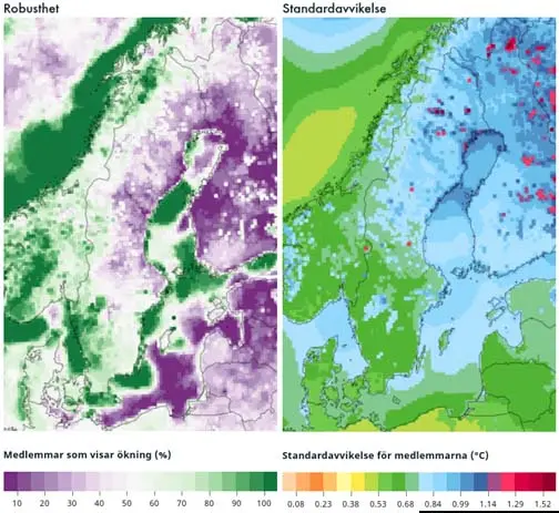
Figure Text:Robustness (left) measures the proportion of models in the ensemble that show an increase; 100% means all models show an increase, while 0% means no models show an increase. Standard deviation (right) shows the extent of variability among the ensemble members. Higher values indicate greater spread.