These pages present how seas in the vicinity of Sweden may be affected by the climate change during the 21st century. The service builds on reanalysis and scenarios from regional climate models forced with several different global climate models. The horizontal resolution in the regional models is approximately 2 nautical miles (about 3.7 km) in the oceanographic part of the model.
In climate model calculations, assumptions on future changes in the atmosphere and ocean are used. The climate models describe the connections between processes in the atmosphere, on the Earth surface and in the oceans.
The results from the calculations with climate models have here, for seas in the vicinity of Sweden, been further processed and visualized. Results are shown for the period 1975–2100. The climate model projections presented come from different models depending on which variables are shown. The physical variables of the Baltic Sea (temperature and salinity in surface waters) and biogeochemical (dissolved inorganic nitrogen and phosphorus in surface water and dissolved oxygen content in bottom waters) come from runs with the RCO-SCOBI model (Saraiva et al. 2019 a, b). The ice indicators in the Baltic Sea come from NEMO-Nordic which is a coupled ice-sea model (Pemberton et al. 2017, Höglund et al. 2017). Finally, the physical variables of the North Sea come from runs with the coupled model RCA4-NEMO (Gröger et al. 2019).
Future changes for each indicator are presented in an overall map of seas in the vicinity of Sweden. The changes are also presented for each sub-basin according to HELCOM's division of the Baltic Sea. Finally, the changes are presented annually as a time series in relation to historical values, which have been produced through reanalysis which in turn takes observed values into account. Reanalysis data for biogeochemical indicators are not yet presented, but will be included when a method has been developed to compensate for known problems with this data, e.g. too high concentrations dissolved nitrogen (DIN) in the Gulf of Riga. In order to obtain robust results in comparison with historical values, it is important that there are several observation points in each sea area being studied. The sea sub-basins (according to HELCOM) are therefore for this comparison gathered in a total of three different sea areas: the North Sea, the Baltic Proper and the Gulf of Bothnia. For demarcation between sea areas, there are different locations for the boundaries depending on the main purpose. This applies in particular to the area including the Sound, the Belt Sea and the Bay of Kiel and Mecklenburg, where for some indicators there may be large gradients. The scenario service follows the distribution described in the Swedish Marine and Water Authority's regulations HVMFS 2012: 18 (according to the Marine Environment Regulation) which complies with the Marine Strategy Framework Directive (MSFD) in Sweden.
Climate models
Climate models are used to calculate future climate. These are 3-dimensional representations of the atmosphere, the land surface, oceans, lakes and ice. In the model the atmosphere and ocean are divided into 3-dimensional grids, across the surface, upwards, and down into the ocean. To get good results the entire global atmosphere and ocean must be considered. Such models are called global climate models. The time evolution of different oceanographical parameters are calculated in each cell of the grid.
Climate models create enormous amounts of information and requires therefore large amounts of computer power, which means that the amount of grid boxes in the 3-dimensional grid must be restrained. The grid in a global climate model is sparse, which gives less details on the regional scale. For regional climate models the grid covers a smaller area, for example Europe. In that way more detail can be achieved for a smaller region without using too much computer power.
The results from a global climate model governs what happens outside the model domain in the regional model. In that way the regional model also considers what happens outside the domain. In this service one regional climate model for the atmosphere and several for the ocean, forced with several different global models are used. In coastal areas, the ocean requires a higher resolution than the atmosphere. Here, approximately 3.7 x 3.7 km resolution is used for the ocean (the size of the horizontal grid in the ocean) while approximately 25 x 25 km resolution is used for the atmosphere (the size of the horizontal grid above the earth surface).
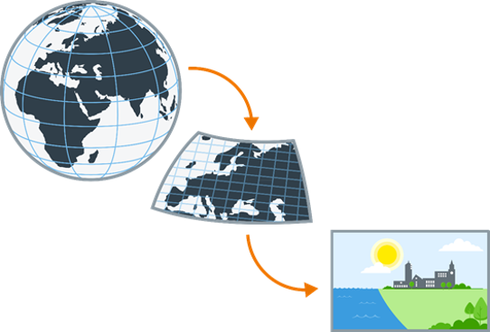
High resolution climate models require large resources, but more details can be achieved by so called downscaling. The higher resolution yields more data points which gives more details, climatological processes are also better described. This applies especially to short lived or local events. Precipitation in general and extreme precipitation in particular is an example of what can be improved by higher resolution. Precipitation may vary largely in space and time. That is better described by a model of high resolution (Rummukainen, 2010; Rummukainen, 2016). In the ocean, higher resolution is for example required to sufficiently describe the flows through narrow passages as the Sound and the Great Belt, which are important for the climate and environment in the Baltic Sea.
Emissions Scenarios
Model simulations of the climate are based on emissions scenarios or radiative scenarios. Emissions scenarios are assumptions of future emissions of greenhouse gases. They are based on assumptions of future development of world economy, population growth, globalisation, transitions to environmentally friendly technology amongst others.
The amount of future emissions is affected by all these factors, which in turn affects the greenhouse effect. A measure of how the greenhouse effect is changing in the future is radiative forcing, measured in power per square metre (W/m2).
The more emissions of greenhouse gases the more radiative forcing. Such scenarios are called RCP scenarios (Representative Concentration Pathways (Moss et al., 2010; van Vuuren et al., 2011)).
In this analysis two scenarios are used:
- RCP4.5: Strategies for reduced greenhouse gas emissions yield a stabilisation of the radiative forcing at 4.5 W/m² year 2100 (used in IPCC, AR5).
- RCP8.5: Increasing greenhouse gas emissions makes radiative forcing to reach 8.5 W/m² year 2100 (used in IPCC, AR5).
For meteorological and hydrological indicators, RCP2.6 is also presented, which is the radiative scenario that is closest to the ambitions in the Climate Agreement from Paris. For oceanographic indicators, there is no complete analysis for RCP2.6 where all indicators are included for all seas in the vicinity of Sweden and analysed with the same ocean model, which is why RCP2.6 is omitted here.
Climate scenarios
A climate scenario is composed of a combination of emissions (or radiative) scenario, global climate model, regional climate model and a time period of choice. See the table in the section on ensembles for more information on the climate models used.
The simulations with regional models start 1975 and the period 1976-2005 is used as reference. Results for the future show anomalies compared to the average of 1976-2005.
Since the results are provided on a grid, so called gridded data, it can be difficult to directly compare model results and observations. Observations give the conditions at a specific point, whereas the models give the average for the entire grid cell. The description of observed climate in this service is based on gridded reanalysis data (a sort of blend of observational and model data) and can thus more easily be compared to climate model data.
Nutrient scenarios
As a complement to the climate scenarios for the Baltic Sea, model simulations for different nutrient scenarios are also presented:
- Base: Corresponds to an inflow of nutrients to the sea in the order of the current level, i.e. the concentrations of nutrients in the water inflow from land do not change over time. The amount of nutrients that reach the Baltic Sea therefore only depends on the climate's impact on run-off (which depends on the amount of precipitation etc).
- Low: Corresponds to a reduction in the inflow of nutrients, which by 2020 has reached the level corresponding to what the Baltic Sea countries previously agreed within the cooperation in HELCOM, the so-called Baltic Sea Action Plan (HELCOM, 2007, 2013).
- High: Corresponds to increases in concentrations of nutrients in the water and atmospheric supply, representing e.g. regional changes in population growth, agricultural practices and sewage water treatment plants. The load of nutrients to the sea is thus affected both by lifestyle and by the impact of climate change on run-off from land.
Data based on observations
In addition to data from regional climate models, the service also contains comparable time series based on observations. In order to be able to compare observation data with data from climate models, the observations are used in a regional reanalysis that has been performed at SMHI for Copernicus Marine Service (CMEMS). The reanalysis is a historical three-dimensional simulation of the sea, considering information from oceanographic observations, both at the surface and at depth. The advantage of using the reanalysis is that the climate variable obtains realistic values with the help of observational data. CMEMS reanalysis is performed with the coupled physical-biogeochemical model NEMO-SCOBI and has the same resolution as the regional climate models for the ocean. Reanalysis data for biogeochemical indicators are not yet presented, but will be included when a method has been developed to compensate for known problems with this data, e.g. too high concentrations dissolved nitrogen (DIN) in the Gulf of Riga. This analysis can be downloaded from Copernicus' Marine Service (CMEMShttps: //marine.copernicus.eu/).
Scenarios are not forecasts
The results from projections made with climate models presented here are called climate scenarios, they are not forecasts. Climate scenarios are based on assumptions of future emissions and amounts of greenhouse gases. They represent the statistical behaviour of the weather of a longer period of time - that is the climate. A forecast, on the other hand, provides information about what will happen in the near future.
Indicators
Oceanographic and biogeochemical indicators are quantitative measures based on observed measurement values and/or data calculated with models. SMHI uses indicators as a basic tool for analysing the state of the environment and for illustrating and communicating changes. Usually an indicator has a unit.
| Name | Definition | Unit |
|---|---|---|
| Surface temperature |
Average temperature in the upper 0-9 m |
°C |
| Surface salinity |
Average salinity in the upper 0-9 m |
PSU |
| Maximum ice extent |
Maximum distribution during an ice year (Sept.-Aug.), area in line plot |
%, km2 |
| Ice thickness |
Average ice thickness (Jan.-April), ice volume in line plot |
m, km3 |
| Bottom oxygen |
Medium acid content at the bottom |
ml/l |
| Surface nitrogen (DIN) | Average content of DIN (nitrate + ammonium) in the upper 0-9 m (Dec.-Feb.)* |
µmol/l |
| Surface phosphorus (DIP) |
Average content of DIP (phosphate) in the upper 0-9 m (Dec.-Feb.)* |
µmol/l |
* Average concentration of dissolved inorganic nitrogen (DIN) and phosphorous (DIP) are only shown during December-February since these concentrations are the ones that influence the algae blooms during the rest of the year.
Reference period
A 30-year period is used to describe the current state (climate and nutrient supply) in the ocean. The period must be long enough so that a significant part of the natural variability averages out. The time period 1976-2005 was chosen since this period had the latest available forcing data when the analyses were performed.
Calculations for the end of the century
The years 2071-2100 represents ‘the end of the century’, to get a uniformity between the constituent disciplines of meteorology, hydrology and oceanography although the oceanographic simulations do not extend to the end of December 2100, but to the end of December 2099 for most models and 2097 for one. In practice, however, it is a minor problem if some ensemble members do not cover the entire time period as there are only a few years missing from the ensemble members and this is assumed to have a marginal impact on the ensemble average value for 2071-2100.
About ensembles
What is an ensemble?
An ensemble is a collection of model scenarios, or ensemble members. The members in the ensemble can differ regarding the driving global climate model, the regional climate model, the emission scenario, or nutrient scenario.
Why should one use model ensembles?
An ensemble provides an overview of the spread in the future climate scenarios and nutrient scenarios. The spread informs about uncertainty in the results, which is important for assessing the robustness and reliability of the information. The reliability of the result increases if several models produce a consistent result.
The role of the climate model
The climate models, both global and regional, will provide different responses to the forcing from a given emissions scenario. These differences arise due to the models’ differing approaches to simulate different physical processes in the climate system, which relate to our incomplete understanding of many processes and our ability to numerically simulate them.
The global climate models determine the main climate sensitivity, and the large-scale atmospheric and oceanographic circulation. They will therefore have the largest impact on the simulated large-scale climate, such as wintertime mean temperature. Other processes are determined at smaller scales, such as summertime precipitation which arise from local cloud processes, where the regional climate models to a large extent dictate the results (Kjellström et al., 2018; Sørland et al., 2018). This may in turn affect the wind over the ocean and the water exchange between inland seas and the open ocean.
It is challenging to select a single best performing climate model, because the models differ in performance depending on the region, the variable and season studied. Including several models increases the robustness and quality of the ensemble mean result, and the most common approach is to include as many models as possible in an ensemble.
Another kind of ensemble can be configured by making several simulations with a single global climate model, where the initial conditions at the start-up of the model leads to different results. This is an effect of the chaotic development of the atmosphere and ocean, which in itself leads to a spread in the results, which is related to the natural variability of the climate system.
Ensembles describe the reliability of the results
The spread within the ensemble provides information on the reliability of the results. The set-up of the ensemble can describe different uncertainties, such as model uncertainty or natural variability.
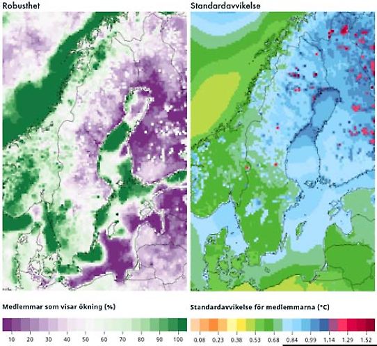
This service presents two measures of robustness and model spread: the relative number of models that show and increase, and the standard deviation across the model ensemble.
The relative number of models that show and increase, presents the model agreement on the sign of the change. If most models agree on an increase, the result can be considered robust. Further, if most models disagree on an increase, it means that they agree on a decrease. If the models show little agreement on the sign of the change, the result is either not robust, or there is no significant change to be expected from the studied variable. The latter requires further investigations.
Standard deviation is a measure of the model spread. Even a robust signal can have significant spread when the magnitude of the change is uncertain. A large spread results in a large value of the standard deviation relative to the magnitude of the change.
The time period matters
The number of models and scenarios to include in an ensemble partly depends on the time period studied. Generally, for the near future (a few decades into the future), the initial conditions influence the results and demands a large ensemble of different model and different initial states. At longer time horizons, the emission scenarios become more important than the initial conditions, but also the sensitivity of the climate model to the greenhouse gas forcing plays a large role.
Natural variability is important in the short-term perspective
The climate system has it’s own natural variability in addition to anthropogenic effects. These natural fluctuations between years, or between decades complicates the analysis of calculated climate scenarios. Especially when studying climate change in the near-term future. The natural variations of the climate cannot be exactly predicted (for example for a certain date). However, it is possible to study natural variability by creating an ensemble of several climate scenarios based on one emissions scenario, but with different initial conditions. By the end of the century, the largest uncertainty in results comes from the choice of climate model, the choice of emissions scenario, and for biogeochemical indicators the nutrient scenario as well.
Models used in this service
The principle is to use as many model simulations as possible, since more data give a better statistical foundation. It is also desirable with ensembles that do not lean too much on specific models. In that case certain models get a disproportionate significance. It may also be desirable that the RCP ensembles are of comparable sizes. The supply of simulations of RCP8.5 is significantly larger than for the other RCPs. There are also model combinations that have only been run for one or two RCPs. Since we want as big ensembles as possible, we will have to accept that the ensembles are not containing exactly the same models. Global models used by only a small number of RCMs and for only one RCP are omitted so that they do not contribute to the skewness between the ensembles.
Ensembles in the oceanographic part of the service are based on the simulations performed in connection with previous research projects. For the indicator’s oxygen, dissolved inorganic phosphorus and nitrogen, data from the RCO-SCOBI model was used (Saraiva 2019a, b). In order to be able to see possible interaction with the indicator’s temperature and salinity, data for these indicators are also taken from the same model. However, this model does not include the North Sea. Therefore, for this area, temperature and salinity indicators have been taken from model RCA4-NEMO (Gröger et al. 2019). At the border between the North Sea and the Baltic Proper, some differences in the results may therefore be seen. Regarding the ice indicators, the analyses have been performed using data from NEMO-NORDIC (Pemberton et al. 2017, Höglund et al. 2017). Despite differences in models, an ensemble composition regarding global climate models (GMCs) that is as consistent as possible has been sought, see the table below.
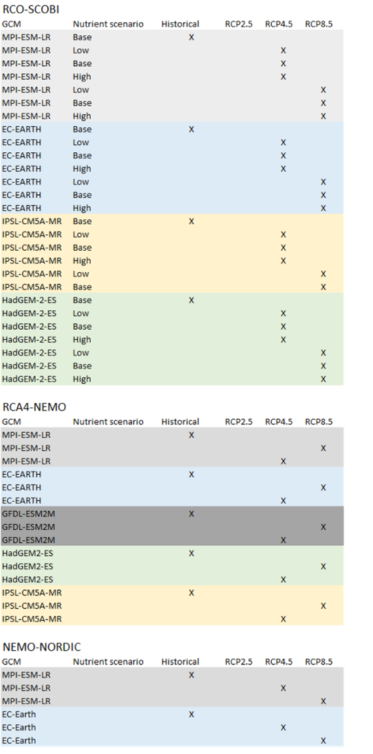
MPI-ESM-LR: Max-Planck Institute Earth System Model LR, https://www.mpimet.mpg.de (Block and Mauritsen 2013, Stevens et al. 2013)
EC-EARTH: European Community model, https://www.knmi.nl (Hazeleger et al. 2012)
IPSL-CM5A-MR: Institut Pierre Simon Laplace Climate Model – Medium Resolution, http://icmc.ipsl.fr; Marti et al., 2010; Hourdin et al., 2013).
HadGEM-2-ES: HadleyCenter Global Environmental model, https://metoffice.gov.uk (Jones et al. 2011)
Robustness of the results
Robustness is here a measure of how certain or uncertain the climate change signal is. Since the results are based on several different simulations with climate models it is possible to do statistical analyses of how robust (i.e. reliant) the results are. Here, two measures of robustness are used: the relative number of models that give an increase and the standard deviation.
The relative number of models that give an increase is a measure of how large part of the ensemble that agrees on a positive change. The greater the share of models that point in the same direction, the more robust is the result. If all models in the ensemble give a temperature increase that is, for example, a robust result. It is also a robust result if no models give an increase. The result is not robust if, on the other hand, the models are relatively equally spread between increase and decrease. One example is shown in the left figure below. Dark green colours imply that most models agree on an increase. Outside the coast of Norway, for example, the relative number of models that give an increase is 100 %; a robust signal. Purple colours imply that most models do not give an increase. In parts of Finland no models give an increase (0 % give increase); that is also a robust signal but of a decrease.
Another measure of the robustness is the standard deviation. It shows how large the spread of the change (signal) is between the models. The standard deviation is large when the spread is large, and small when the spread is small. The value of one standard deviation means that ca 68 % (if the results follow a normal distribution) of the models are within that value. The spread is relatively small in southern Sweden and northern Finland in the example to the right below.
Ice indicators have no figures for robustness and standard deviation since only two members are included in the ensemble.